Chances Created is a metric which tries to quantify the number of goal scoring opportunities that a player is directly involved in. Opta definition is Assists + Key Passes, where Assists are passes (final touch) which result in a goal from the subsequent play and KP are passes which result in a shot that doesn’t become a goal. So chances created can be reduced to the final passes (touches) before another player has an attempt at goal (and scores or doesn’t). As I’ve discussed on podcast The Monthly Football Podcast, Assists alone are pretty random since you rely on the shot actually going in the goal, so chances created is a bit less noisy and should more reliably predict future assists than assists actually do due to the sheer volume of chances created and opportunities for goals to be scored rather than relying on goals actually being scored which is hard.
Chances created relies on a player to actually have a shot at the end, otherwise there is no record of the opportunity. Opta also have ‘Chance Missed’, which is defined as a big chance opportunity where the player doesn’t get a shot away. Chance missed will be attributed to the player who has the big chance and decides not to shoot, which doesn’t help the creator who provided the chance. If we assume that the miss is largely due to the player not executing an attempt, then mapping these chances missed back to the creator in addition to chances created would give credit to creating the opportunity and not punishing them for something out of their control, such as the forward deciding to delay a shot and missing the chance to.
Chances Denied Metric
As usual, chances created and most quantified statistics deal with the offensive side of the game since it’s more tangible. Shots are there and they happen, counting them is pretty straightforward. A bit less straightforward is to count the passes prior to shots, with chances created. Both of these can be tracked over many events and quantify expected outcomes based off similar situations in the past, this results in expected goals and expected assists. What is not straightforward is how to quantify the benefit of defensive actions.
We can count tackles, blocks, interceptions and recoveries, however, much like steals, blocks and rebounds in the NBA, they don’t quite tell the whole story about how a defence works. Weaker teams are asked to defend more since they have less possession, this means they have more chances to rack up interceptions, tackles and recoveries. Possession adjusting these measures helps somewhat to normalise these differences, which means that we can compare the frequency of each action assuming they all have equal chances to do so. However it’s still hard to differentiate the quality of the actions, or how important they were to each team.
Chances denied are an attempt to quantify how much of an opportunity was denied by an interception or ball recovery. In a purely defensive, denying your opponent a goal scoring opportunity, sense, recovering the ball in the middle of the pitch is not as important as recovering the ball on the edge of your own box. Expected threat, created by Karun Singh (@karun1710), is a metric which quantifies how likely a team is to score from each location on the pitch within the next 5 actions. If we assign the xT to a recovery or interception or tackle considering the location on the pitch it occurs then we may get a proxy for how important each action was. Since defensive teams will get more opportunities, it may be worth possession adjusting this also to compare like for like.
The general concept trying to be captured here is to quantify the quality of chance or potential quality of chance that is denied due to the action taken by the defender. This quantity can be given solely to the defender making the action or collectively assigned to the players involved to appreciate the team aspect of defensive play. There is a question whether to include tactical fouls in here as well as legal ball recoveries, but will save that for another time.
After attending StatsBomb’s Introduction to Football Analytics last week, I was inspired to take another look at the free events data that they offer. One of the main obstacles to breaking into the football analytical industry is getting data to play around with and show what you can do, which is why Statsbomb’s commitment to offering such samples of data for free is so amazing and should be taken advantage of! There are endless possibilities of insight and visualisations to create using the event data, limited only by your creativity.
Support and free tutorials are also freely available for using data in R, including their own StatsBombR package and FCrStats’s twitter and GitHub who provides functions for creating custom pitches for visualisations. Did I mention they were both free?
It can be intimidating to start to work with complex data like this, so I will go through step by step and create a version of a popular match visualisation: an Expected Goals Shot Map.
Since the Fifa Women’s World Cup is currently taking place and the StatsBombR package is continually being updated with new games as they are played, I thought I’d use the recent England v Argentina game as an example.
Install RStudio
FOr those completely new to R, you can download the latest RStudio version here:
library("StatsBombR") # Event data
library("SBpitch")    # Custom functions for creating pitches
library("ggplot2")    # Building visualisations
library("tidyverse")  # Data manipulation
Create Blank Pitch
Using FCrStat’s SBpitch package you can create a pitch to use with custom visualisations using the create_Pitch() function. You can specify the colours and which lines you want to see. For the xG Shot Map, we will use the whole pitch.
Using the StatsBombR package, getting access to the free events data is as simple as running the StatsBombFreeEvents() function as below and storing it in your environment.
statsbomb_events <- StatsBombFreeEvents()
## [1] "Whilst we are keen to share data and facilitate research, we also urge you to be responsible with the data. Please register your details on https://www.statsbomb.com/resource-centre and read our User Agreement carefully."
Get Match Info
There are over 100 variables for each event of each match, so we want to narrow the data set down to a single match. We are interested in the Fifa Women’s World Cup match with England v Argentina. We are also only interested in shots, so will only include those types of events.
I have also included the colours for the respective teams to use later on.
The x,y location of each event is stored in a single variable as an array. Using the separate() function in the Tidyverse we can extract these and create new variables called “location_x” and “location_y”. Use as.numeric() to make the new location variables numeric so we can plot them later.
event_type <- "Shot"
team1_colour <- "red4"
team2_colour <- "lightblue"

# Narrow down to a specific match: Australia Women's v Brazil Women's
match <- statsbomb_events %>%
  filter(# Fifa Women's World Cup Competition ID
           competition_id == 72 &
           # Eng Womens v BArg Women's Match ID
           match_id == 22962 &
           # Only keep events that are shots
           type.name == event_type ) %>%
  # X,Y locations are stored in a single array column, separate() into two columns
  separate(col = location, into = c(NA, "location_x","location_y")) %>%
  mutate(location_x = as.numeric(location_x),
         location_y = 80 - as.numeric(location_y))
Create Goal and xG Indicators
Since we are interested in the actual goals and expected goals of each shot, we can create a goal indicator variable and respective expected goal variables for the shots of each team.
match <- match %>%
  mutate(# Create a goal indicator
         Goal = ifelse(shot.outcome.name == "Goal","1","0"),
         # Create England goal indicator and xG
         team1_Goal = ifelse((shot.outcome.name == "Goal" & team.name == unique(match$team.name)[1]),"1","0"),
         team1_xG = ifelse(team.name == unique(match$team.name)[1],shot.statsbomb_xg,NA),
         # Create Argentina goal indicator and xG
         team2_Goal = ifelse((shot.outcome.name == "Goal" & team.name == unique(match$team.name)[2]),"1","0"),
         team2_xG = ifelse(team.name == unique(match$team.name)[2],shot.statsbomb_xg,NA)
)
Plot Shot Locations
Okay, lots of preparation done so far. Let’s plot some shots!
ggplot2 builds plots from the ground upwards. Remember the blank_pitch we made earlier? We use that as a base and add the shot locations on top using geom_point to add points/dots
Oops, looks like all the shots happened at the same end, regardless of team. We need to reverse the shot locations of one team, since we know the pitch dimensions from create_Pitch() as 120 x 80, we can use those.
# Looks like all shots are at the same end, need to reverse the locations of one team
match <- match %>%
  mutate(location_x = ifelse(team.name == unique(match$team.name)[1],
                             120 - location_x,
                             location_x),
         location_y = ifelse(team.name == unique(match$team.name)[1],
                             80 - location_y,
                             location_y)
         )
Plot Respective Coloured Locations
Let’s see if it worked!
# Try again, with different colours for each team
blank_pitch +
  geom_point(data = match, aes(x=location_x, y=location_y, colour = team.name)) +
  theme(legend.position="none") +
  scale_colour_manual(values = c(team1_colour, team2_colour))
Oof, looks like England had lots of shots and denied Argentina anything significant.
Highlight Goals
We have shot locations, but it would be nice to see which shots are goals using the goal indicator we created earlier and we can use a different shape (triangle) to differentiate.
Looks like England scored from their shot closest to the goal in the Argentina 6-yard box. Let’s see how likely they were to score by using the size of the points to reflect the expected goals.
Looks like England scored with their best chance and could potentially have scored a few more considering their volume of relatively good shots. This is a skeleton of an Expected Goals Shot Map, we can add in annotations to make the final plot look more presentable and quantify each team’s expected goals versus actual goals.
That looks a little better, at least we now know the score and how each team did compared to their expected goals. After creating a blank pitch, we only need to add layers to get a visualisation of the information we want which is incredibly powerful. To get the visualisation for another match, simply change the match_id (and team colours) above!
The only packages used to create this are those loaded above, with the free events data provided by StatsBomb and extra functions/tutorials by FCrStats
Again, you can find those two here: @StatsBomb @FCrStats
Hopefully this will help get some people get started and overcome any initial intimidation. I will look to provide more of these types of step by step guides going forwards the more I get to play around with the data.
Manchester City find themselves once again top of the Premier League, with the chance to retain the title for the first time in 10 years since Manchester United in 2008/09. However they also find themselves without Fernandinho, the only seemingly irreplaceable player in their squad that overflows with talent. Fernandinho has missed four Premier League games so far this season, the two at the end of December in which they lost and left the league title in Liverpool’s hands and the two most recent games which were both dominating 1-0 wins. Even if their performances were no worse off and just lacked some luck, no doubt there is nobody else in their squad who can do exactly what Fernandinho does.
Even Guardiola has commented that there is no doubt they will be looking to bring in a replacement:
“I think with the way we play we need a guy who has of course physicality, is quick in the head and reading where our spaces to attack are”
Guardiola
In this post I will try to scout a replacement for Fernandinho using Statsbomb’s 2018 FIFA World Cup Event data. This is a small sample size, so will only include players and their performances in the World Cup. I will define some metrics that could be used to describe the type of player that would fit the role that Fernandinho plays and identify those players that performed best during the World Cup.
Guardiola talks about physicality, quickness of thought and reading where the spaces will be to attack. It is hard to quantify those qualities, however using adapting some simpler metrics could give a good shortlist.
We know that Manchester City will have the ball a lot and want to get the ball forwards to their more attacking players in attacking areas, relying on Fernandinho to progress the ball. Using Statsbomb’s passing events, with the start and end location in x, y coordinates, I have defined a ‘Progressive Pass’ to be one that moves up the pitch more than 10m. Players who have the ability to progress the ball forwards are desired. It could be argued that we also want to only include players who progress the ball from deeper positions so as to more accurately emulate Fernandinho’s role, however we have a small sample as it is and the ability to play progressive passes is what we are looking for.
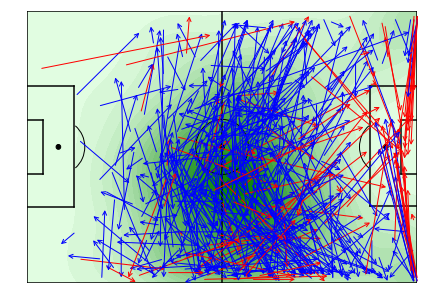
Whilst lots of players are great at passing, what makes Manchester City so special and Fernandinho so hard to replace, is their ability or willingness to win the ball higher up the pitch. Check out a previous post in the link below where I show how many more times they win the ball back in the opposition’s half. In the same vein, using Statsbomb’s ball recovery event with the x, y location I create a count of times that a player has recovered the ball in the opponent’s half. This tries to emulate the ability to win the ball back quickly after losing it and pinning the opposition back.
The combination of progressive passes and high ball recovery is used as a proxy for the type of skills that Fernandinho portrays and can be used to get a shortlist of players that perform similarly. Looking at only the players who played positions considered as central midfield or defensive midfield, the top 10 is below.
Figure 1: Midfield Progressive Passes and Opponent Half Recoveries Top 10 from 2018 FIFA World Cup
One thing to note is that these are pure counts and not per game or per 90min. It would be worth taking a look at that to account for the differences in games and minutes played. For example, Croatia making the Final and Germany getting knocked out in Group Stage is a difference of four games, so Toni Kroos making it to 2nd on the absolute list is incredible.
Initially it looks like the list makes sense, players like Kroos, Modric, Rakitic are all players who you could see being able to play in a deeper midfield role. Mascherano is also in the same mould, even more so considering he has played at Centre Back most of the time for Barcelona and Fernandinho has begun to slot in there to bring the ball out.
Those players are all 30+ years old so no better than Fernandinho in terms of potential replacements. Granit Xhaka and Marcelo Brozovic are two that are just entering their prime midfield years at the age of 26. This is where it’s important to note that when scouting, context is important and large sample sizes are encouraged. Xhaka may have the progressive passing ability and love of yellow cards, but probably wouldn’t have the discipline.
This post has looked at outlining a way to narrow down a shortlist of potential replacements for Fernandinho, the methods can be used to find similar players for any player as long as you can identify what you are looking for. Ideally you would get a much larger sample size of games and could look at a player’s contribution per game or per 90mins to get a more stable shortlist. In the future I would like to look at some unsupervised methods which don’t require you to specify or create the similar fields as I have done here.
I have included the total passing heatmaps and the recovery maps of selected players; if you want to see any players specifically from the World Cup from any position then give me a shout!
Once again, massive shout out to Statsbomb for providing the free source of event level data, it’s hard to come by and even harder to collect so it’s much appreciated!
I will take a look at the intriguing situation that Deportivo Alaves have found themselves in. Comparing where they were a year ago to where they are now, I will look to identify whether or not their current results are sustainable.
In 2016/2017, Mauricio Pellegrino managed Alaves to 9th place in their first season back in La Liga for 6 seasons. This was a great achievement and quickly drew the eyes of the Premier League where he went on to manage Southampton. Luis Zubeldia, an Argentine who had never managed in Europe before, took over for the start of the 2017/2018 season before being sacked after losing and failing to score in each of the first four games. Gianni De Biasi, who was previously the Albania coach who managed to qualify them to their first major tournament, replaced Zubeldia. Though he managed to get them their first goals and wins, it wasn’t enough as after only two months in charge his contract was terminated as Alaves sat rock bottom of the La Liga table on 6 points. They had 2 wins and 11 losses from 13 games, only scoring 7 goals and conceding 22. After a great first season back in La Liga finishing 9th the year before, this wasn’t exactly how they’d hoped the start of their second season would go. Since then, Abelardo Fernandez has been in charge and has won 19 out of 35 La Liga games, winning 1.74 points per game. Alaves would’ve finished 5th in the 2017/2018 season had they maintained that across a season and qualified for Europe. After 10 games in the current 2018/2019 season, Alaves find themselves 2nd only behind Spanish giants Barcelona.
Apart from the set back early in 2017/2018, Alaves have proved they are well worth their place in La Liga. In only their 3rd season back to La Liga they are sitting in 2nd place, I will take a look at the stats behind their recent fixtures to judge how sustainable their recent results have been.
So far Alaves have won 6 games, drawn 2 games and lost 2 games, meaning they are at 2 points per game and results are better than average across Fernandez’ tenure. They have scored 14 goals and conceded only 9, however their expected goals (xG) is 10.41 and expected goals against (xGA) is 13.59. Alaves are outperforming their expected returns at both ends of the pitch, they are scoring more than and conceding less than is expected based on the shots that have occurred. When a team is outperforming their expected goals, it is usually not sustainable, elite level finishing is the exception. We can expect that Alaves will regress back to the mean, wherever that mean is.
Even though Alaves have outperformed their xG/xGA as a total, looking at each match they’ve played individually tells a different story. Since they appear to be over performing expectation, you may expect that they over perform in each game. This is not the case as there is only one game that they have won where they had a lower xG than their opponent (1.10 – 0.85 vs Real Valladolid [away]). This includes their win against Real Madrid in which they snatched victory in the last-minute to earn a 1-0 win with xG of 0.95 – 0.84.
Two games in particular highlight the importance of looking at individual games, their first game away to Barcelona and their away trip to Rayo Vallecano. Barcelona thrashed Alaves 3-0 on the opening day after receiving a guard of honour for winning the title last year, with xG of 3.27 – 0.25. So 3.27/13.59 of xGA and 3/9 of their goals against all came in the first game, in the nine games since then they have had an xG of 10.32 and conceded 6. They are still out performing xGA, however it’s a much more representative view. Several games later, Alaves won 1-5 away to Rayo Vallecano with xG of 1.08 – 1.25. Helped out by a Rayo Vallecano red card and some excellent finishing in the first half, they created some higher xG chances in the second half with more space to counter into and ran away with the game. There were 5/14 of Alaves’ goals but only 1.25/10.41 xG in this game, meaning that in the other nine games they had and scored nine goals from 9.16 xG which looks much more reasonable and sustainable.
Across each individual game the xG prediction for a winner is correct 70% of the time (2 draws and 1 loss), if Alaves carry on putting up these numbers for xG and xGA then there’s no reason why their success isn’t sustainable. The only question is whether they can keep it up. Of course, xG doesn’t win you games, actual real-life goals do. Let’s delve into what type of goals and when these goals are scored.
Alaves haven’t scored a single goal in the middle 15 minutes of any half (15-30/60-75mins). This means all of their goals have come at the start or the end of a half, these are very good times to score. A goal at the start of a half will put you on the front foot and a goal at the end of the half gives the opposition little time to react, if it’s just before half time you can go and regroup whilst if it’s just before the end of the game there’s usually no time for reply. It is not a conscious decision when they decide to score but provides insight into the flow of how Alaves try to play. Explosive starts to each half with a quieter middle to relax before ending strongly. Alaves are very good at finishing halves but whether that style of play is sustainable is another matter, out of the 10 games they’ve played in they have scored in 90+ minutes five times. This has won them three games and drawn one meaning that they have gained seven points from last-minute goals. That is not sustainable.
Considering that Alaves appear to be over performing their expected returns at both ends at a total level, the fact that they have scored goals in 90+ minutes in half of their La Liga games and they are currently sitting at 2 points per game which is above their average in the last year, it doesn’t appear that their current results are sustainable. That’s not to say that they will revert back to the relegation battling side a year ago, but they will regress back to their mean somewhere in between.
Credit to understat.com once again for their amazing site and xG models. Check them out.